Using whole genome SNP data, PLINK
software offers a
powerful and simple
approach to population stratification. This includes genome-wide
identity-by-state (IBS) counts for all pairs of individuals. Each SNP
locus
presents 3 possible states: none of the alleles matches (IBS0), one
allele
match (IBS1), and both alleles match (IBS2). For each pair, the
frequency of
occurrence of these states (freq1, 2 and 3, respectively) can be
estimated by
dividing these counts by the total number of loci for which genotypes
were
determined in both individuals. Clustering of pairs according to the
degree of
kinship is clearly revealed when plotting these results in three
dimensions
(3D) (Fig. S1).
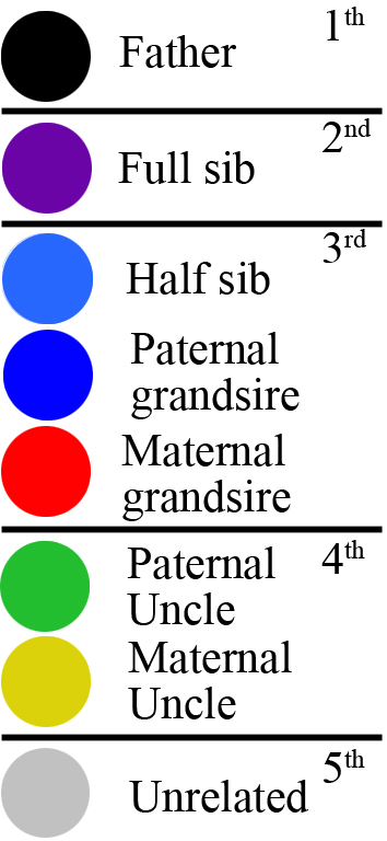
Fig. S1. Kinship within the population of
Israeli artificial
insemination (AI) bulls- 3D plot. Using
SNP50 BeadChip data of 789 sires, the genome-wide identity-by-state of
each
possible pair of individuals is illustrated by plotting a colored dot
at the 3D
coordinates that correspond to the frequency of the 3 possible states
of the
SNPs’ alleles (freq0- no match, freq1- single match, freq2- both match).
Dot
colors indicate the familial relation and kinship level according to
the
following key.
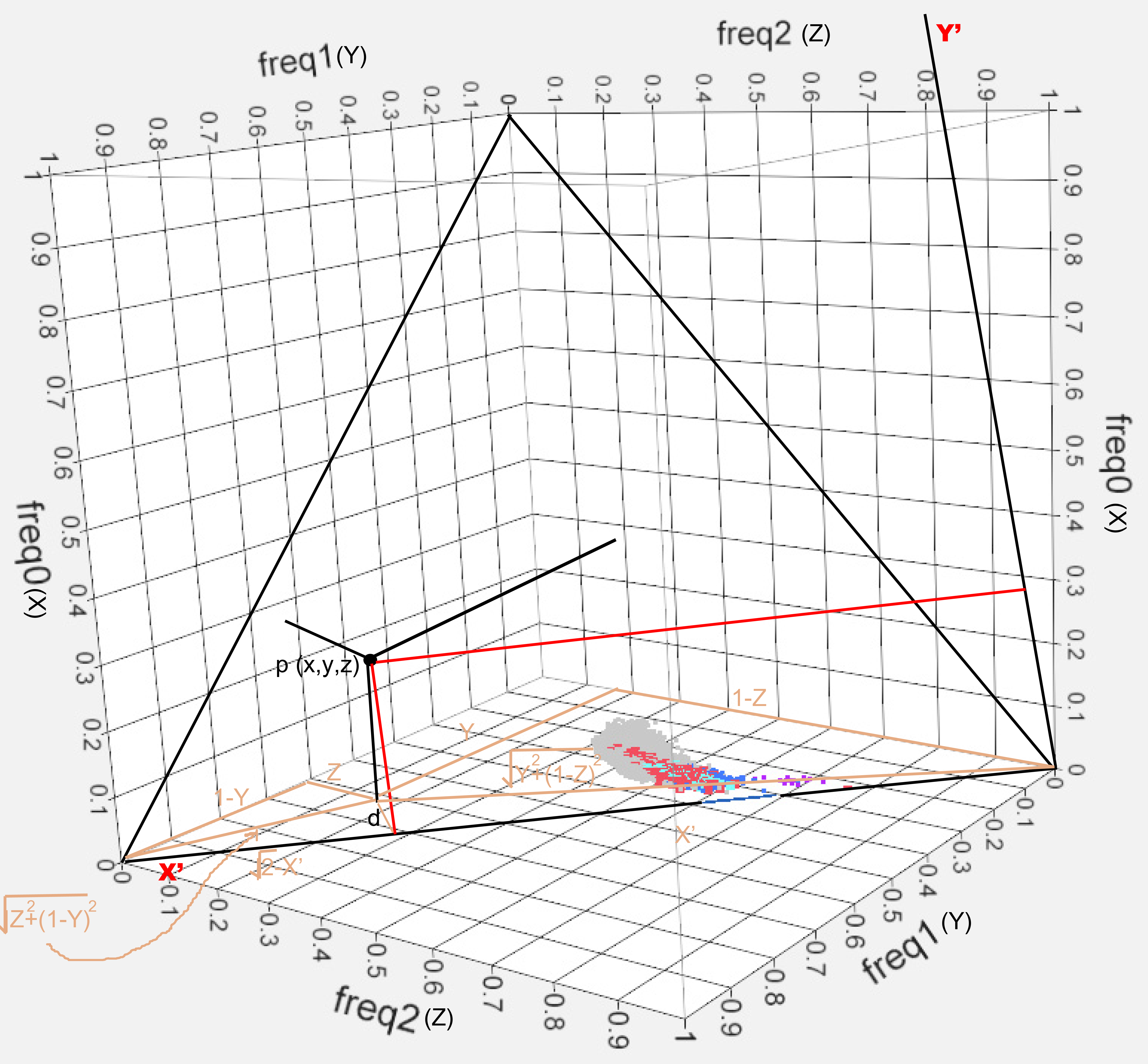
Fig. S2. Cartesian coordinates on kinship data
plane. Axes (X’, Y’) were
fitted to the plane formed by the frequency of
the 3 possible states of the SNPs’ alleles for the data
described in
Fig. S1. The point P has coordinates x, y and z (black) which correspond to
coordinates x’, y’ on the fitted axes (red).
Eq. 1 d2=z2+(1-y)2-(√2-x’)2=y2+(1-z)2-x’2
z2+1-2y+y2-2+2√2x’-x’2=y2+1-2z+z2-x’2
2√2x’-x’2+x’2=y2+1-2z+z2-z2-1+2y-y2+2
2√2x’=2-2z+2y=2(1-z+y)
Eq. 2 x’=0.7071(1+y-z)
Eq. 3 x’=0.7071(1+freq1-freq2)
Y’ is inferred from the
right
triangle with base d and altitude x (Fig. S2) using the sine function.
Eq. 4 y’=x/sin(54.7o)=1.2247x
Eq. 5 y’=1.2247freq0
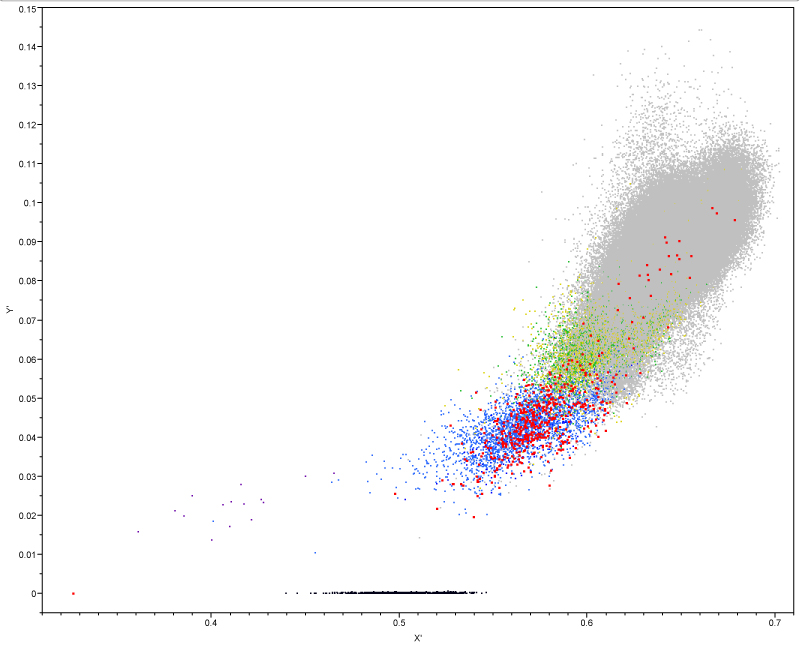
Application of equations 3 and 5 to
the BeadChip 3D data of the Israeli AI sires (Fig. S1) projects this
kinship illustration
onto a bi-dimensional plain (Fig. S3).